Predictors
Predictors work just like aggregators except that they return a time series that represents the future of the series it is applied on.
To get a more complete understanding of the different type of aggregators, please refer to the whitepaper RD5.
Three predictors are currently implemented:
Least squares
Holt
DLM
DLM
DLM Stands for Dynamic Linear Models. It is the easiest and most reliable predictor out of the three, and should thus be preferred in most situations.
However it can however be very intensive in terms of computing power: the complexity of this algorithn increases exponentially with the number of samples used in the prediction. The maximum number is limited by the skyminer.dlm.max_datapoints property of the configuration file.
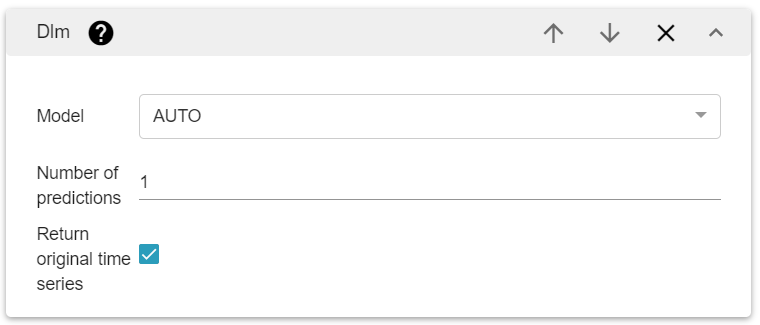
It has three parameters:
The number of predictions to be performed. Interval between predictions depends on the regularity of your data and is automatically assessed.
The name of the model that is used for the prediction. It must be one of
AUTO,
DETERMINISTIC_LINEAR,
DETERMINISTIC_EXPONENTIAL,
STOCHASTIC_LINEAR,
STOCHASTIC_EXPONENTIAL,
RANDOM_WALK,
GENERAL
A boolean to show the time series with the predictions or not.
Holt
Holt hestimated the local trend of the timeseries, and can tolerate any amount of data with any regularity. The downside is that the smoothing parameters must be evaluated manually, making this algorithm hard to use for inexperienced users. Finally it can only predict one sample, as predicting more than one wouldn’t be relevant.
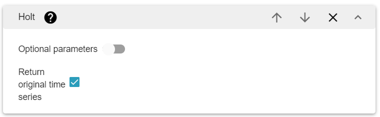
It has three parameters:
The level, which indicates how weight is balanced between the previous samples and those before.
The slope.
A boolean to show the time series with the predictions or not.
Least Squares
Least squares estimates the global trend of the timeseries, and can tolerate any amount of data with any regularity.
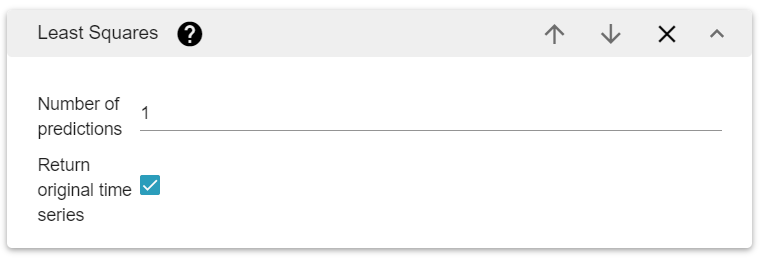
It has two parameters:
The number of predictions.
A boolean to show the time series with the predictions or not.
Advanced
DLM
All the implemented models are designed to extract a periodic pattern and a trend.
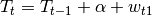
Thus the state space is always of the dimension of the period, with one element Tt and p-1 elements St.
The dynamic equation modelling seasonality remains the same through all models:

It is very important that used data is structurally regular (consistent sampling rate) with possibly some missing values. If data sampling is irregular, it will be rejected by the processor. The aggregation tools offered by Skyminer allow you to easily prepare data in an appropriate manner.
See the section on data requirements for more precise information.
Parameter Estimation
Defining a dynamic linear model is only the first step. The core of the pattern matching is actually the parameter estimation.
For a given period p, parameters α, ϕ, w_t1, w_t2 et v_t are estimated with a powerful trust region algorithm called BOBYQA, created by Powel (Powel, 2009). This algorithm tolerates simple constraints which is very interesting as we would like to avoid estimating negative variances with the algorithm. Even if it is an efficient optimisation algorithm, our problem is strongly non-convex and thus good initialisation of parameters is crucial.
The periodic nature of the sequence must be assessed. As per the model, for a period of length p the state contains p-1 variables S_t in charge of estimating the values of the function during the period. If periods become large, this implies a very large state space, and thus very heavy computations. Moreover parameter estimation must be realised for each period length. To keep computational time reasonable, two techniques are employed:
Sparse matrix computation, which allows to keep the complexity of a matrix/vector product linear and matrix/matrix product quadratic.
Multiscale period evaluation. The idea is to evaluate the quality of the period length parameter for long periods first on a downsampled version of the data. Only the best period is selected and assessed on the finer data. This avoids optimising the parameters for every single period length between 2 and the maximum period length, and more importantly it limits the number of long period evaluations.
The last step is to select the most appropriate model.
Several models are available… Trend estimation is what makes the difference between models.
General Structural
Name: GENERAL_STRUCTURAL

This is the most general model, using 3 parameters only for the trend. This model would have the best adaptability to many different data structures, but it also often provides false detections of trends and thus is very prone to overfitting. The use of this model should thus be avoided as much as possible. Also it is important to notice that the more parameters there are, the more difficult the optimisation and thus the more likely it is that the parameter estimation will not result in the best combination of parameters possible.
Stochastic Linear
Name: STOCHASTIC_LINEAR_PLUS_SEASONAL
The stochastic linear model sets the value of the exponential trend to 1, thus disabling it. It will detect a linear trend that tolerates some deviations thanks to the noise parameter w_t1. Some examples can be easily found where this kind of model overestimates the presence of linear trends because the noise parameter gives it too much liberty. It must also be used with care.
Deterministic Linear
Name: DETERMINISTIC_LINEAR_PLUS_SEASONAL
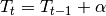
The deterministic linear model tries to detect only a linear trend and does not allow the level to fluctuate around it. Everything that is not a periodic pattern or linear trend will thus be considered as measurement noise. This model lacks a little bit of flexibility because data that does not follow a constant or linear trend will be poorly estimated.
Random Walk
Name: RANDOM_WALK_PLUS_SEASONAL
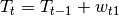
This is the classical random walk trend that allows the trend to freely fluctuate in any direction. The pattern estimation will thus only focus on periodical pattern extraction to give the better prediction possible. This is considered as a good combination with the deterministic linear model, in the case were the second one fails to detect a clean linear trend.
Exponential models
Name: STOCHASTIC_EXPONENTIAL_PLUS_SEASONAL and DETERMINISTIC_EXPONENTIAL_PLUS_SEASONAL
and

These models should only be used if an exponential trend is known to exist. The testing of exponential models has shown that these were too unstable for forecasting. Even a very small error in the estimation of ϕ has important consequences even on medium horizon forecasting. For instance a value of 0.99, which is close to 1 and can easily be generated by noise or outliers, makes the trend drop at 60% of its value in only 50 samples of forecasting. This is very unpleasant for the robustness of the algorithm.
Automatic model
Name: AUTO
Automatic model tries to pick up the best fit between Random Walk and deterministic Linear. On purpose models that have a general worse fit (like exponential) are not evaluated.
Data requirements
The data provided to the predictor must comply with some basic requirements. The format of the data accepted forces it to be regularly spaced in time. The number of missing values must remain reasonable, both in proportion and distribution throughout the data. Indeed the downsampling propagates missing values. Trying to infer them would introduce a strong bias into the downsampled sequence. Thus periodically distributed missing values might interfere with the periodic pattern estimation and the prediction will fail.
A maximum number of about 200 samples should be considered for the input data. The periodic pattern estimation becomes less reliable and computationally more expensive when it becomes too long. It seems more reasonable to realize proper aggregation before trying to apply the analysis. Indeed the resolution of the forecast that one might expect logically depends on the time span of the data used and the length of the desired prediction. For instance, if one wants to predict the values that will occur in the next 5 hours, it seems very unlikely that the knowledge of data that dates back to a few months ago would be useful. Also it is statistically unrealistic to try to predict the behaviour of the data during 5 hours with a precision up to 1 millisecond. Also it is often unrealistic to expect a prediction that is longer than the data to be of any significance. Predicting on more than the half or the third of the length of the data should be avoided or used with great care. A minimum number of sample has also been set by default because the model is invalid with period length smaller than 2. Thus if the minimum number of repetition for the pattern is 3, the minimum number of samples will be 6. Of course in most situations trying to extract a pattern on a set of 6 samples will not make sense.
Note
Example of procedure that maximises the prediction tool efficiency:
Choose the date at which you would like to start your prediction.
Choose the time span of the prediction you wish to make.
Compute the length of the data to be considered for the prediction. It should be at least a few times longer than the prediction time span.
Aggregate so the length of the considered data is represented by less than 200 samples.
The resolution of the prediction being the same as that of your data, compute the number of sample to predict.
Apply prediction!
References
Chatfield, C. (2003). The Analysis of Time Series: An Introduction. Chapman & Hall/CRC.
Hanzak, T. (2014). Methods for periodic and irregular. Prague: Charles University.
Jalles, J. T. (2009). Structural Time Series Models and the Kalman Filter: a concise review. Cambridge.
Powel, M. (2009). The BOBYQA algorithm for bound constrained optimization without derivatives.
Shumway, & Stoffer. (2011). Time Series Analysis and Its Applications. New York Dordrecht Heidelberg London: Springer.
Holt
Computes the holt exponential smoothing prediction. Holt is a variation that involves double exponential smoothing. Holt is considered as a good trend estimation tool that can adapt to any data irregularity, but it does not model periodic patterns.
References
Cipra, Tomáš (2006) - Exponential smoothing for irregular data. (English). Applications of Mathematics, vol. 51, issue 6. https://dml.cz/handle/10338.dmlcz/134655
Chatfield, C. (2003). The Analysis of Time Series: An Introduction. Chapman & Hall/CRC.
Least Squares
Least squares prediction simply uses a least squares linear regression over the data time period (data fitting using a straight line).
This gives a simple trend that is extrapolated by the algorithm. Indeed periodic patterns are not taken into account by this model.
Provides a very fast but low accuracy prediction
References